Preliminary operation

Before continuing and understanding how to create a pivot table, it is good to spend a few words on the use of tables of this type, without neglecting the format of the worksheet from which one should start.
Exactly as I mentioned in the introductory lines of this tutorial, a pivot table is an "alternative" method to reorder the data already present in a spreadsheet: in fact, it is possible to use a pivot table to obtain a quick summary, but complete, of the information at your disposal, with the possibility of ordering and combining them according to the aspect that must be taken into consideration, without upsetting the structure of the initial spreadsheet.
In other words, a pivot table offers the possibility of analyzing at a glance the data contained in a spreadsheet without having to learn how to use formulas and macros: just to give you an example, given the set of operating expenses of a home, you can generate a pivot table to view "on the fly" the expenses for each month of the year and for each reason (bills, medical expenses, education, and so on), instead of manually adding - and based on the chosen category - the elements of each column.
In order for the program (in this guide we will use as examples Microsoft Excel e LibreOffice Calc) is able to generate a pivot table containing exact data, the data in the starting spreadsheet must be well structured and meet a series of very specific conditions, which I am going to list below.
- If the PivotTable is to contain headers, the worksheet must also contain headers.
- Le header lines, if present, they must immediately precede the data lines, without any separation.
- In the starting spreadsheet, or at least in the range of data for which the pivot table is being built, there should be no blank lines.
- The data contained in the columns must be homogeneous, so that they can be combined (added, subtracted, multiplied, sorted, counted and so on) when creating the pivot table. This means, for example, that in a hypothetical "Amount" column there should be only and only numerical values, relating to amounts in the chosen currency.
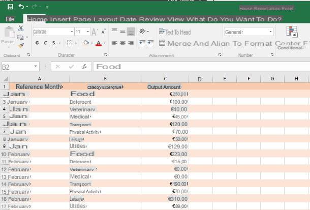
In later parts of this tutorial, I will refer to a spreadsheet containing an expense statement for monthly household expenses: the column A contains the month reference, the column B la category of the outlet and, finally, the column C contains the relative amount in euros.
As for the versions of the programs, in this guide I will refer to Microsoft Excel 2016 and LibreOffice Calc 5, both running on the platform Windows. The same instructions, however, can be safely used on previous / subsequent versions of the aforementioned programs or on operating systems other than Windows, for example MacOS.
Create a pivot table with Microsoft Excel
You have it available Microsoft Excel to manage your spreadsheets? Then this is the section for you: in the following lines I am going to provide you with all the instructions you need to create and manage a pivot table using the application produced by Office.
To get started, double-click the Excel file containing the data to be processed, making sure the spreadsheet meets the requirements listed above. If, on the other hand, you need to start from a new file, start Microsoft Excel, click the icon Blank workbook, then fill the created document with the data you want to enclose in the pivot table. If you want to better customize your new spreadsheet, I suggest you refer to my guide on how to use Excel to find a series of useful tips.
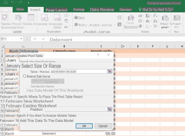
Now that your spreadsheet is ready, you can proceed to create the associated pivot table: select, by dragging the mouse, thedata range you intend to process (or click inside any data cell to process the entire worksheet), presses on the item Inserisci placed at the top and then on the button Pivot table, resident on the left.
At this point, on the screen that opens, put the check mark next to the item Select table or range (if necessary), make sure the box Table / Range contains all the cells of the table (or of the chosen data range), put the check mark next to the item New worksheet e pulsing sul pulsating OK. The game is done: Excel will automatically open the new worksheet (you can go back to the previous spreadsheet at any time using the tabs located below) prepared for data processing through the pivot table.
Note that the table headers (e.g. Reference month, Category e Exit amount) now become i fields of the pivot table, to be arranged and organized according to what you want to achieve.
Operate on the table
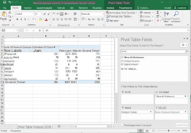
Before arranging the fields inside the newly created pivot table, let me give you some general hints on organizing this type of tables. A pivot table, exactly as shown by the Excel window, is mainly made up of three areas of interest: the area Riga, the area Column and the area Values.
Generally speaking, it can be said that the non-numeric fields (in our example, the expense categories) are arranged in the area Riga, fields containing data, ore o reference periods are arranged in the area Columns, while the fields numeric (usually those that need to be combined with mathematical operations) are added to the area Values. However, it must be said that the arrangement of the fields in the areas of a table of this type varies greatly depending on the type of "summary" to be obtained and the scenario in which the analysis is carried out.
Having made this necessary premise, it's time to add the fields to the newly created pivot table: identify the area Pivot table fields located to the right of the Excel screen, then select one of the available fields with the mouse (eg. Reference month) and drag it to the most suitable area of the table (eg. Columns), and then repeat the operation for all the fields you intend to analyze. In this example, the field Expense category will be added to the area Lines and the field Exit amount to the area Values, so as to obtain a complete view of the total expenses related to each month.
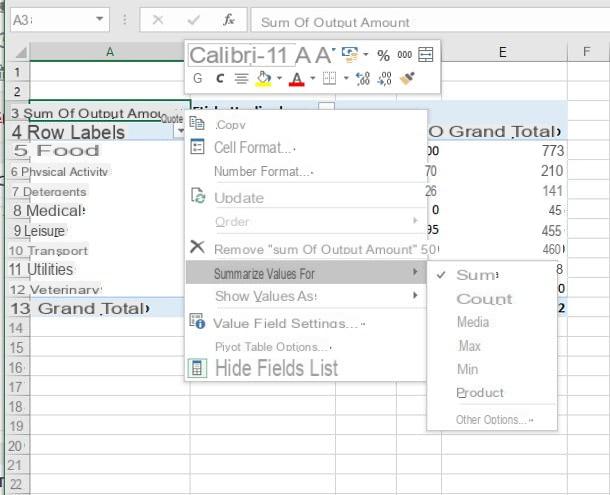
By default, Excel PivotTables do the Sum of the data contained in the field Values, if these are numeric, or the Count if they are textual or inhomogeneous; if you wish, you can change this behavior by right clicking on the cell Sum of [Column Name] in the pivot table, and then selecting the item Summarize values for from the menu that appears on the screen. At this point, you just have to choose the arithmetic operation you want to perform on the data contained in the value field (minimum, maximum, average, and so on).
If you wish, instead of displaying the values in currency (or in any other type of numeric format), you can choose to display them in percentage: in the example we are analyzing, this would be very useful for studying the category with the highest percentage of expenses. . To proceed, right click on the summary cell of the values (eg. Sum of Import Output) and select the items Show values as>% of grand total.
Of course, you can use the value format that suits you best and move the fields within the various areas as you like, until you get the view you want: this is precisely the strength of pivot tables! Finally, I want to remind you that the pivot table updates automatically when values belonging to the data range included in the processing are added, removed or modified: if the update operation was not immediate, you can click on the button Update attached to the panel Pivot table fields and located at the bottom right.
If you've made it this far, it means you have all the information you need to build a pivot table using Microsoft Excel. However, I want to remind you that the possibilities of this program do not end there: just to give you some examples, you can generate graphs and histograms, overlap them to create even more precise statistics, create more or less complex tables to manage the sorting of data and much, much other. In short, the potential of this software is by no means limited!
Furthermore, I would like to point out that you can edit files created with Excel even on platforms other than Windows and macOS: the software is in fact available, albeit with some limitations, as an app for Android, iPhone and iPad (free for devices up to 10.1 ″) And as a web application that can be used directly from the browser.
Create a pivot table with LibreOffice Calc
You don't use Microsoft Excel to manage your spreadsheets, but instead refer to LibreOffice Calc? Don't worry, you can easily create pivot tables using this software! Also in this case, the rules relating to the construction of the spreadsheet as seen in the section relating to preliminary information are valid: the data must be homogeneous, sorted and they must not be present blank lines.
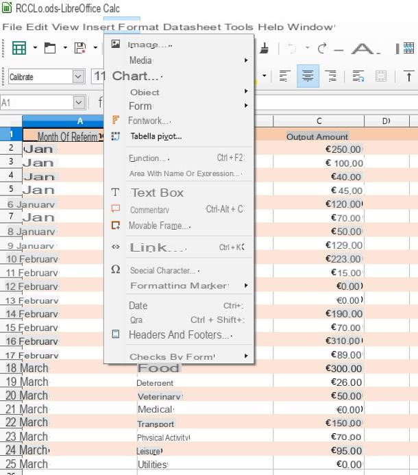
That said, it's time to get down to business: open the spreadsheet containing the data to be processed in LibreOffice, or build one by strictly following the rules mentioned above. Once this is done, select with the mouse the data range on which to operate (including headers) or click on any cell of the range to analyze the entire table, then press the menu Inserisci located at the top and select the item Pivot table ... da quest'ultimo.
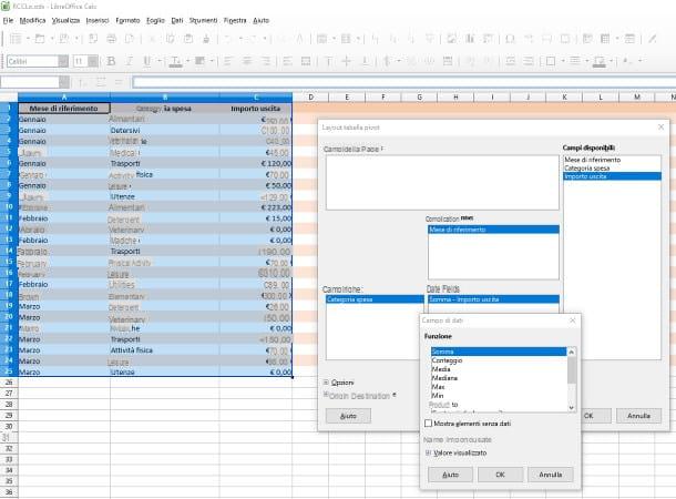
Once this is done, put the check mark next to the item Current selection in the small panel that opens, presses the button OK and, following the same rules that I suggested in the section relating to Microsoft Excel, arrange the fields of your worksheet (eg. Reference month, Expense category e Exit amount) in the fields of the corresponding pivot table (Row fields, Column fields e Data fields).
Again, the default operation on numeric data fields is sum: to change this behavior, double-click on the corresponding item (eg. Exit amount) and select the desired operation (sum, count, median, average and so on) from the checkbox Function, then pressing on OK but I will complete the operation.
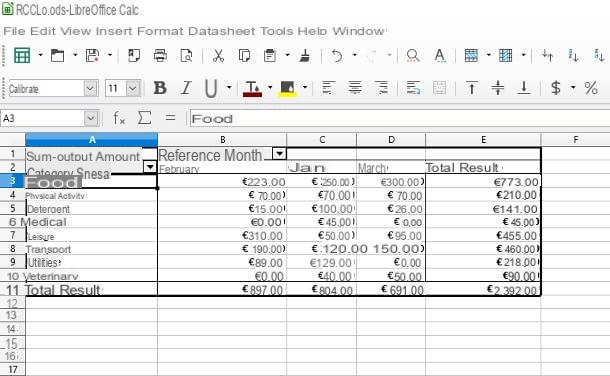
To finalize the creation of the pivot table, all you have to do is click on the button OK: immediately afterwards, the program displays the new sheet containing the table resulting from the previous operations, which you can customize graphically using the handy side box that opens on the screen.
Remember that, using the procedure described above, you can create all the views in the pivot table you want: simply return to the spreadsheet, using the tabs located at the bottom left of the Calc screen, and repeat the operation by changing the arrangement of the various fields.
How to create a pivot table