Simple list
As already mentioned above, the Excel drop-down menus can contain values defined directly by the user - therefore phrases, words or figures present exclusively within the menu - or values already present in other areas (or other pages) of the spreadsheet. calculation.
To create the first type of drop-down menu, the one containing values defined directly by the user, you must select the cells in which to insert the menu and click on the button Data validation located in the tab Data Excel (top right). If you can't find it, it's the icon that looks like two white text fields: next to the first is a green check mark and next to the second a red prohibition sign.
If you need help selecting multiple cells at the same time, just click on the first cell to include in the selection; then you have to keep the key pressed Uppercase (Shift) on the computer keyboard and click on the last cell to be selected (provided that you want to select a range of cells belonging to the same column or row). To select cells "scattered" in various rows and columns you have to use the combination Ctrl + click on Windows and the combination cmd + click your Mac.
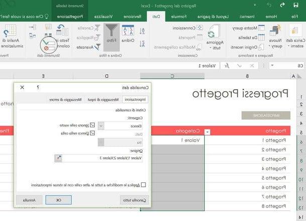
Now you have to define the values to appear in the drop-down menu. In the window that opens, select the item List from the menu Allow and type, in the field Origin, all the options you want to see in the menu (separating them with a semicolon). For example, if you want items to appear in the drop-down menu Value 1, Value 2 e Value 3, in the Excel Source field you have to type Value 1; Value 2; Value 3.
At this point, pigia sul pulsating OK to save the settings, select any of the cells where you have entered the drop-down menu and you will see a small one appear arrow on the right. Click on this arrow and you will see a menu appear with all the options you previously specified in the field Origin of Excel.
Subsequently, to change the options available in the drop-down menu, select the cells of your spreadsheet again, click on the button Data validation Excel and change the values in the field Origin.
Drop-down menu with values taken from the spreadsheet
Now let's see how to create Excel drop down menus using values already present in the spreadsheet.
The first step you need to take is to select the cells that contain the data you want to include in your drop-down menu. The cells must be arranged on the same row or column (with no gaps between one cell and another).
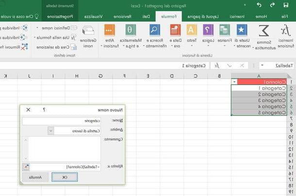
When done, select the tab Formulas Excel and click on the button Define name located at the top right (the white label icon). In the window that opens, type the name under which you want to group the values you have just selected (eg. category if you have selected a list with various product categories, giorni if you have selected a list with all the days of the week and so on) and click on the button OK per salvare i Cambiomenti.
Finally, select the cells where you want to insert your drop-down menu, go to the tab Data Excel and click on the button Data validation located at the top right (the icon of the two text fields with the green check mark and the red prohibition sign).
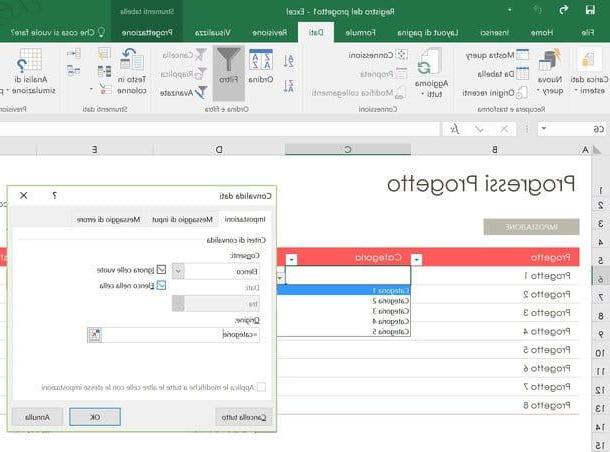
In the window that opens, select the option List from the menu Allow and type, in the field Origin, the name of the data group you selected earlier, preceding it with the "=" symbol. For example, if you want to create a drop-down menu with the values of the "days" group you have to type = days, while if you want to create a drop-down menu with the values of the "categories" group you have to type = categories. Pulia quindi sul pulsating OK and you will see a drop-down menu appear in all the cells you have previously selected.
Now try to guess: what will the drop-down menus that appear in the cells of your spreadsheet contain? Exactly! All the values of the cells that you grouped at the beginning of the procedure.
Another very interesting thing to underline: by changing the values present in the cells grouped at the beginning of the procedure, the items present in the drop-down menus are also modified. All completely automatically. Convenient, right?
If you want, you can also edit the groups of cells that were previously grouped and add or remove values from them. To change the range of cells that is part of a group, select the tab Formulas Excel, click on the button Name management and double click on the name of the group to edit. In the window that opens, click on the icon of Red Arrow (bottom right) and define the new range of cells to include in the group.
Have you changed your mind and want to delete a previously created drop-down menu in Excel? No problem. In case of second thoughts, you can remove the drop-down menus from the Excel cells by simply selecting the latter by clicking on the button Data validation located on the tab Data of the program (top right) and pressing the button Erase everything present in the window that opens.
How to create drop-down menus in Excel